MICHAEL HASEY // AI & ARCHITECTURE

Image Synthesis Study 1

Automating Prokudin-Gorskii Photo Collection Colorization

Overview

This study proposes a computational method to autonomously colourize the Prokudin-Gorskii Photo Collection, which is a series of black and white photographs of the Russian Empire taken by Sergei Mikhailovich Prokudin-Goirskii in the early 20th century. In addition to being grayscale, each photograph is in fact a montage of three copies of the same image stacked one above the other. Each copy within the montage represents one of the three channels of the RGB color spectrum. The images are stacked with the blue channel image on top, the green channel image in the middle, and the red channel on the bottom.

The aim of this study was to use image processing techniques to autonomously and efficiently split the image into its three parts, align and stack them correctly to produce a colour image, and apply efficient coding methodologies and techniques such as image pyramiding to complete this task in a very short period of time when applied to very large images.

Original Prokudin-Gorskii Photo Collection plates. Notice the 3 images in each plate. The top image represents the blue channel, the middle the green channel and the bottom the red channel.

Step 1: Splitting the Image into individual RGB Channels

To begin, the image must be split into its three RGB channel components (red, green, blue). Simple image manipulation methods are conducted to split regions based on height/3 then assign to new variables. A false color filter has been added to the images below to better illustrate the specific RGB channel associated to each image.

Step 2: Cropping images

As evident in the three RGB channel images above and in the original grayscale plates, the Prokudin-Gorskii photos contain irregular black borders and are not always centered in the image. As a result, split images contain traces of this border which may seriously impede alignment efficiency. In order to crop borders, a simple algorithm is used to remove a certain percentage of pixels from each side of the image. A standard 5% pixel removal is set, but this can be respecified by the user.

Step 3: Aligning Images

Image alignment is a tricky problem that can solved in a number of different ways. Before attempting to align the Prokudin-Gorskii Photo Collection, I undertook a series of experiments testing various alignment methods with simpler images and models. See “Additional Experiments” below. However, two general methodologies can be used for image alignment that work well for this application.

METHOD 1: SSD

The first and simplest method is finding the sum of square differences (SSD) - also known as the L2 norm - between the images. This method simply compares the average sum of pixel values between two images and returns the difference. As a result, a SSM value of 0 means that the images compared are the same and aligned perfectly. And thus, lower SSM values correspond with images that are more aligned, and higher SSM values correspond with images that are less aligned. In order to find the lowest SSM value and best alignment location, I used the numpy function np.roll to shift single images within a range of possible locations. These possible locations are confined within a pixel range specified by the user. For example a 15x15 pixel range, would result in the image being slightly shifted 225 times within that range. Once shifted, the SSD value would be calculated again. Once all shifts have been made, the shift with the lowest SSD value is chosen and applied to the image in order to achieve the best shift and thus, alignment. In this study, both the green and red channels were shifted via this method to align with the blue channel. Though this method worked well with some images (see image to right), I soon discovered that it was fairly inconsistent and slow with many misaligned image results (see below).

An example of a successful alignment using the SSD method.

MISALIGNED SHIFTS: Though the SSD method worked for the above image of the icon above, it did not always work well with the other images. This perhaps was caused by higher contrast between the separate RGB images within the original plates which co… — MISALIGNED SHIFTS: Though the SSD method worked for the above image of the icon above, it did not always work well with the other images. This perhaps was caused by higher contrast between the separate RGB images within the original plates which could have made alignment through pixel value comparison more challenging. Another issue may have been the specified search area size being used. In above images, a 70x70 pixel alignment search area was used. Perhaps a smaller search area could have improved results.

METHOD 2: NCC

The second method is called normalized cross-correlation (NCC), which scores image alignment via the dot product between two normalized vectors. Like the SSD method, I aligned the Red and Green channels with the blue channels by cycling through a range of possible displacements by using the np.roll function. However, opposite to SSD a higher score indicates better alignment while a low score indicates less alignment. After implementation, I achieved better results with more correct alignments. However, certain images (ie. the “Emir” image) continued to present problems and was not able to be aligned. All other images were successfully aligned nonetheless.

The NCC method aligned images much more successfully than the SSD method. Below are the pixel shifts required for alignment as well as the pixel search area and total process time. These are reduced sized images and are approx. 830x720.Left Image:… — The NCC method aligned images much more successfully than the SSD method. Below are the pixel shifts required for alignment as well as the pixel search area and total process time. These are reduced sized images and are approx. 830x720.
Left Image: Search area: 50x50 pixels Time: 148 seconds. Green shift: [19,7] pixels. Red Shift [44,9] pixels
MIddle Image: Search area: 30x30 pixels Time: 25.9 seconds. Green shift: [14,3] pixels. Red Shift [28,2] pixels
Right Image: Search area: 30x30 pixels Time: 24.9 seconds. Green shift: [11,1] pixels. Red Shift [22,8] pixels

NP.ROLL FUNCTION

np.roll() is a numpy function that shifts array elements, in this case image array elements, along a specified axis. By shifting all array elements (pixels) in an image, we can incrementally and slowly shift an image around and then determine whether a new alignment is better aligned to the base image via the SSD or NCC method. See gif image to right for an illustration of the np. roll function as applied to a simple 2x3 array. Notice the 1 value is incrementally shifted around the array. For more complex arrays with more values, all individual elements would incrementally shift as well.

array_np.roll.gif

Step 4: Processing Large Images Quickly

In step 3, it was determined that the NCC method produced the most accurately aligned images. Thus, I decided to apply the NCC algorithm to the full size image plates. However, I soon realized that the sheer size of the image (3741x9732 pixels, 83.6 MB) compared to the smaller test images previously used (923x2400 pixels, 4.5 MB) was extremely taxing on the algorithm and slowed the alignment process down immensely. As a result, automated colourization on the full-size image plates would not be feasible with NCC and np.roll alone (even when applying this process to the small images, it took approx. 25 seconds on average to complete, still a quite long processing time for a fairly simple task.) To speed up the alignment process for large, full-size images, I constructed a recursive “Image Pyramid” framework which dramatically reduced processing time to around 6 seconds per image.

WHAT IS AN IMAGE PYRAMID?

Image Pyramids allow typically process heavy and slow functions to be rapidly carried out on images that have been downsampled / reduced in size. Structurally, an image pyramid exists as a series of downsampled images that represent progressively lower resolution versions of a larger target image. To situate this in space, one can imagine the smallest and lowest resolution image at the top of the pyramid and the largest and highest resolution image at the bottom. A series of other image copies exist in between and reduce in size and resolution as they travel up the pyramid. Image pyramids are unique as they allow typical process heavy functions to be quickly carried out on the smallest image, with results being upsampled and applied to the largest image. The benefit of this is reduced process time. However, the results of these processes carried out on the smallest images are less precise due to their lower resolution. To achieve more precision, one can move down the pyramid and carry out these processes on higher resolution images, thus increasing precision. However, when operated in conjunction in a recursive manner, the results of one layer can be shared amongst the rest of the pyramid layers, thus incrementally increasing precision overall with the largest gains achieved in the smallest and fastest layers and the smallest and more precise gains being achieved in the largest. As a result, typically process heavy functions applied to large images can be carried out much faster through this recursive image-pyramid method.

credit: wikipedia https://en.wikipedia.org/wiki/Pyramid_(image_processing)

IMAGE PYRAMID APPLICATION

In this study we used the smallest image to conduct the majority of the alignment procedures as it would be the least process heavy means of achieving general image alignment. Once NCC was used to determine the x and y axis shifts need to achieve the best alignment at this resolution, the shifts were then upsampled and applied to the full-size image. The final alignment shift was continuously updated with finer and finer adjustments as the alignment function moved its way down the image pyramid towards the largest full-size image. As it moved down, the alignment function also reduced the search area (ex, 15x15 to 8x8 to 4x4, etc) as the image had already been updated and aligned by the previous, smaller image in the pyramid. By the time the final layer with the largest, full-size image was reached, the alignment procedure has nearly been complete, thus the least amount of alignment searching needs to take place. As a result, the algorithm front loaded the majority of the alignment searching and image shifts to the top of the pyramid where the image is the smallest and thus least process heavy, and the least amount of alignment searching and image shifting to the bottom where processing requirements are high. As a result, implementing reduces the image alignment process on large images to a mere 6 seconds. Resultant images shown below.

displacement: 15x15 Green channel offset: [ 54 , 8 ]Time: 6.89 seconds Red channel offset: [ 116 , 10 ] — displacement: 15x15 Green channel offset: [ 54 , 8 ]
Time: 6.89 seconds Red channel offset: [ 116 , 10 ]

displacement: 15x15 Green channel offset: [ 42 , 4 ]Time: 6.9 seconds Red channel offset: [ 88 , 32 ] — displacement: 15x15 Green channel offset: [ 42 , 4 ]
Time: 6.9 seconds Red channel offset: [ 88 , 32 ]

displacement: 15x15 Green channel offset: [ 56 , 18 ]Time: 6.93 seconds Red channel offset: [ 116 , 26 ] — displacement: 15x15 Green channel offset: [ 56 , 18 ]
Time: 6.93 seconds Red channel offset: [ 116 , 26 ]

displacement: 15x15 Green channel offset: [ 54 , 12 ]Time: 7.2 seconds Red channel offset: [ 112 , 10 ] — displacement: 15x15 Green channel offset: [ 54 , 12 ]
Time: 7.2 seconds Red channel offset: [ 112 , 10 ]

displacement: 15x15 Green channel offset: [ 78 , 28 ]Time: 6.86 seconds Red channel offset: [ 176 , 36 ] — displacement: 15x15 Green channel offset: [ 78 , 28 ]
Time: 6.86 seconds Red channel offset: [ 176 , 36 ]

displacement: 15x15 Green channel offset: [ 40 , 16 ]Time: 7.22 seconds Red channel offset: [ 90 , 22 ] — displacement: 15x15 Green channel offset: [ 40 , 16 ]
Time: 7.22 seconds Red channel offset: [ 90 , 22 ]

displacement: 15x15 Green channel offset: [ 60 , 16 ]Time: 6.89 seconds Red channel offset: [ 124 , 14 ] — displacement: 15x15 Green channel offset: [ 60 , 16 ]
Time: 6.89 seconds Red channel offset: [ 124 , 14 ]

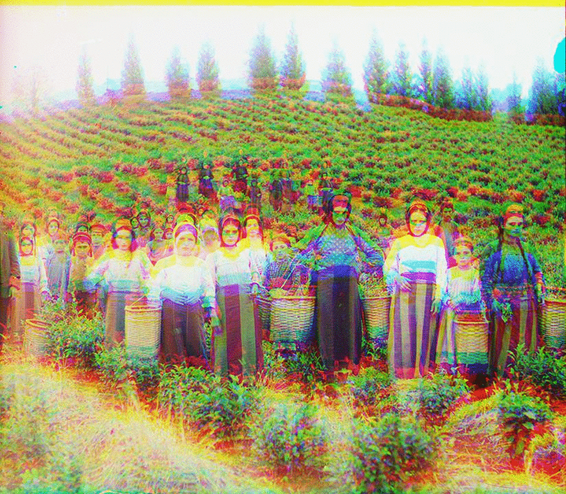
displacement: 15x15 Green channel offset: [ 64 , 10 ]Time: 7.15 seconds Red channel offset: [ 138 , 22 ] — displacement: 15x15 Green channel offset: [ 64 , 10 ]
Time: 7.15 seconds Red channel offset: [ 138 , 22 ]

displacement: 15x15 Green channel offset: [ 48 , 24 ]Time: 6.8 seconds Red channel offset: [ 0 , 10 ] — displacement: 15x15 Green channel offset: [ 48 , 24 ]
Time: 6.8 seconds Red channel offset: [ 0 , 10 ]

Additional Experiments

Before attempting to align the Prokudin-Gorskii Photo Collection, I conducted a series of experiments testing various alignment methods with simpler images and models.

TEST 1: SSD ALIGNMENT WITH SIMPLE IMAGERY

I first wanted to test the basic SSD algorithm with simple geometry to understand the alignment process works. As you can see below, alignment works well with images that have the same color, for example, the image on the left where all three squiggles are black. However, the SSD algorithm has trouble aligning image geometry when the grayscale colours don’t match (image on right). This early realization helped me understand why image alignment with the Prokudin-Gorskii images was so difficult when using the SSD method.

squiggle_plain_np.roll.gif

SSD capable of efficient alignment when images share the same colour or tone.

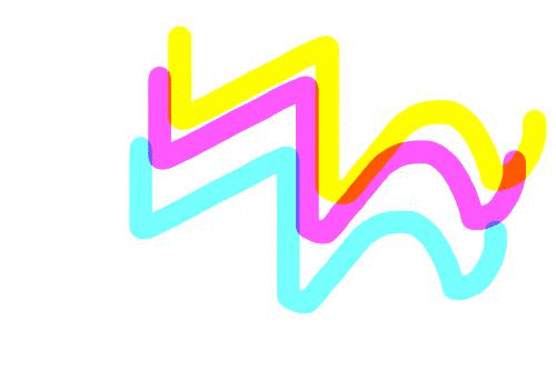
test_2_Squiggle_fade_np.roll_rchan_problem.np_roll.gif

SSD has difficulty aligning channels when colour or tone differs between images.

TEST 2: SSD ALIGNMENT WITH COMPLEX IMAGERY

Test 2 is a repeat of test 1, but instead of using a simple image, a more complex cat image was used. As seen below, SSD again had trouble aligning images with different gradients, colours and tones. I suspected this may have been the result of aligning the wrong rgb channel (green and red) with the wrong base channel (blue), but similar issues were still observed after various recombination efforts. Another issue may have been mislabeled images, aka assigning the lightest gray image as green channel vs blue etc. Again various recombinations did not improve results. Finally, images were arbitrarily lightened in photoshop, thus perhaps causing the misalignment issues as these lightened gradients do not represent a true RGB image representation / transformation.

test_4_Cat_Same.np_roll.gif

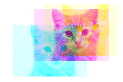
SSD capable of efficient alignment even when complex images share the same colour or tone.

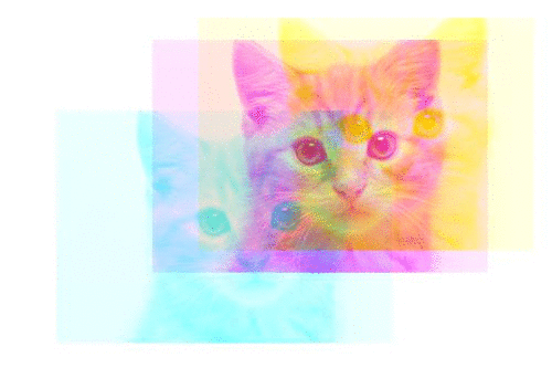
test_6_Cat_Faded_color_reverse_np.roll.gif

Again, SSD has difficulty aligning channels when colour or tone differs between images which is common in the Projudin-Gorskii Photo Collection.