


Deep Vernacular : Analyzing 300+ 3D Wooden Church Forms Using Deep Learning
Graduate Thesis Overview
type: Graduate Thesis Projectyear: 2022school: Carnegie Mellon Universityadvisors: Daniel Cardoso Llach, Jinmo RheeGoogle Scholar Link: Original Publicationkeywords: Deep Learning, Artificial Intelligence, building morphometry, VAE, 3D Dataset Creation, Synthetic Data, 3D Form Analysis, 3D Form Generation, Digital Heritage, Vernacular ArchitectureAbstract
This work explores how artificial intelligence (AI) can help us make sense of the immense variety of architectural styles in the world and how they relate to one another in terms of their geometric similarities and differences. While traditional methods have been limited to analyzing just a few buildings at a time due to their manual and time consuming nature, recent advances in AI technology provide the means to study hundreds, thousands, or even millions at a time. Similar to DNA, these new algorithmic techniques can break down the complexities of 3-D building form into a similar kind of abstracted mathematical representation. This allows an AI system to identify complex features from large collections of building data and shed light into formal aspects of our built environment. For instance, by revealing subtle or difficult to detect form patterns or complex architectural form relationships that would have been challenging or impossible to detect amongst thousands of buildings using traditional methods. Given these new and powerful tools, AI-based form analysis methods have opened the doors to new types of architectural exploration at a massive scale, and can perhaps even change the way we think about architectural form itself.
For this work, we document the creation of a custom dataset of 331 3-D wooden churches located primarily within the Carpathian Mountain Regions of Ukraine and reveal morphological patterns that enhance existing scholarship on the subject. In particular, the complex rules that govern their vast and often entangled range of architectural styles and sub-styles. The dataset construction and analysis process resulted not merely from the implementation of advanced 3-D reconstruction and deep learning techniques, but also — and crucially — from subjective decisions, historical scholarship reviews, and expert and archival engagement. Documenting these, we illustrate how data collection, curation, and analysis are contingent upon social and technological factors, while identifying strengths and weaknesses, and opportunities for architectural-historical analyses to draw from historical traditions and state-of-the-art computational methods.
Indirectly, this paper also demonstrates an alternate means of architectural preservation through a combination of 3-D building reconstruction from sparse imagery and architectural style encoding using DL-methods. When considering the latest threats of war given Russia’s current invasion of Ukraine and targeted destruction of culturally significant buildings, computationally preserving both the churches themselves and their stylistic “essence” becomes increasingly important if we hope to fully document and protect these irreplaceable objects of Ukrainian architectural folk heritage for future generations.
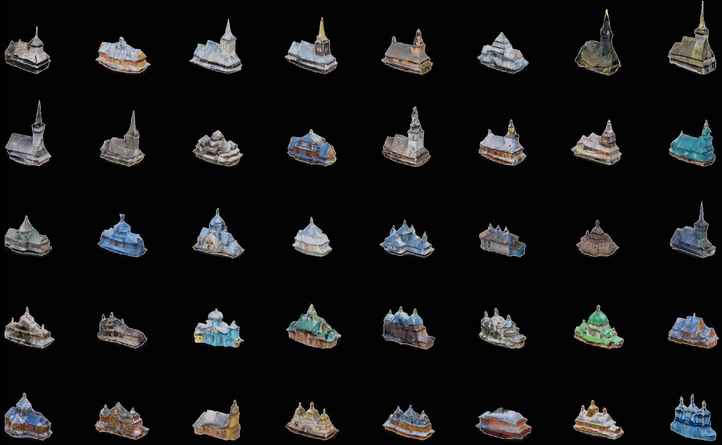
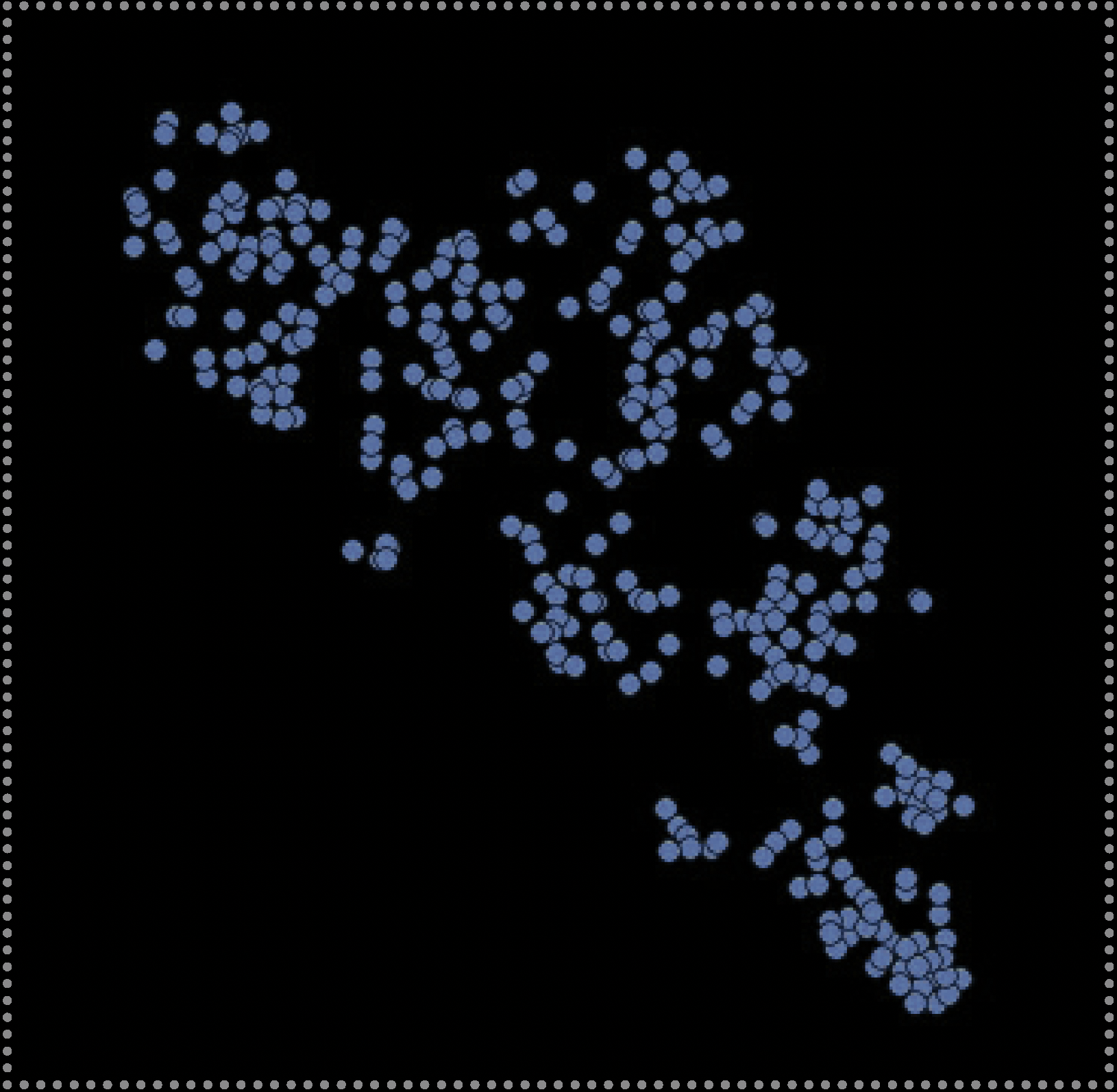
An example of a portion of the training dataset of 3-D churches reconstructed from 2-D images (above) with the entire dataset encoded and represented within 3-D latent space (right). Each point represents a single church’s position in latent space in relation to all others in terms of form. Point color indicates churches that share similar geometric forms, which in turn, may suggest which church style it belongs to. Ex. Boyko, Lemko, Hutsul, or Transcarpathian style.
Research Goals
Create a large dataset of hundreds of digital 3-D Carpathian wooden church models using the NeRS method.
Use Deep Learning to encode & analyze how their diverse range of styles relate to one another in terms of morphological differences & similarities.
Investigate how domain knowledge, geographic data, and reference to existing research and experts can enhance this understanding.
Explore generative methods to synthesize novel 3-D Carpathian wooden church designs using the learned latent feature vectors.
Preface
Big Architectural Data
Today, digital 2-D architectural data in the form of photographic images, maps, and drawings is more prolific and accessible online than ever before. For instance, over 220 billion street-view images covering 10 million miles of roadways now exist on Google Maps, making it possible for us to easily and quickly explore the vast architectural diversity of our world Furthermore, software such as “OpenStreetMap” and Google’s “Open Buildings” have created large-scale urban datasets that record the 2-D building outlines or “footprints” of nearly every building in our world. In combination with other image repositories, these resources provide the foundational data for a new type of architectural research. Onethat aims to analyze thousands of, rather than just a few, buildings at a time.
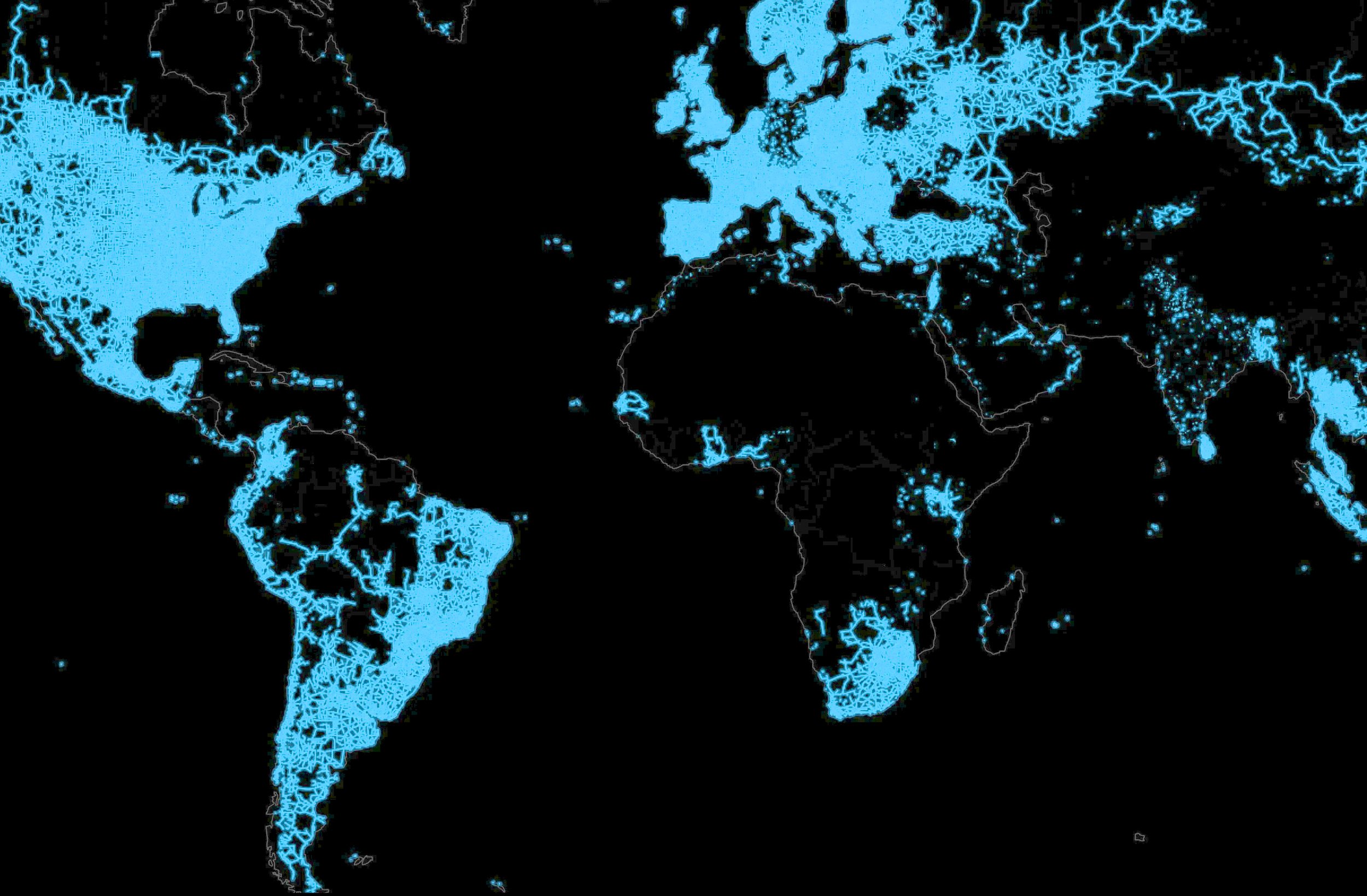
Worldwide Google Street view coverage as of 2019. Over 220 billion images as of 2022.
New A.I.-Based Tools for Architectural Research
Until recently, the majority of architectural form research has focused on just small building datasets at a time due to manual and time-consuming traditional methods. However, within the last few years, architectural form research has experienced a surge in interest, due in part, by the advancements in Deep Learning (DL) based visual pattern recognition tools which provide the means analyze hundreds or thousands of buildings at a time. Early examples of this include a project by V. Moosavi who used DL methods to encode and organize the urban forms of one million cities around the world into distinct form categories and another by Jinmo Rhee, who in 2019 used these methods to identify the various types and locations of urban form patterns throughout the entire city of Pittsburgh, Pennsylvania. By leveraging the analytical power and capabilities of DL, both of these projects were able to obtain results that might have taken years to complete via manual survey and traditional form analysis methods.

1 million cities color coded according to similar urban layout (informed by road network configurations)

Building Typology
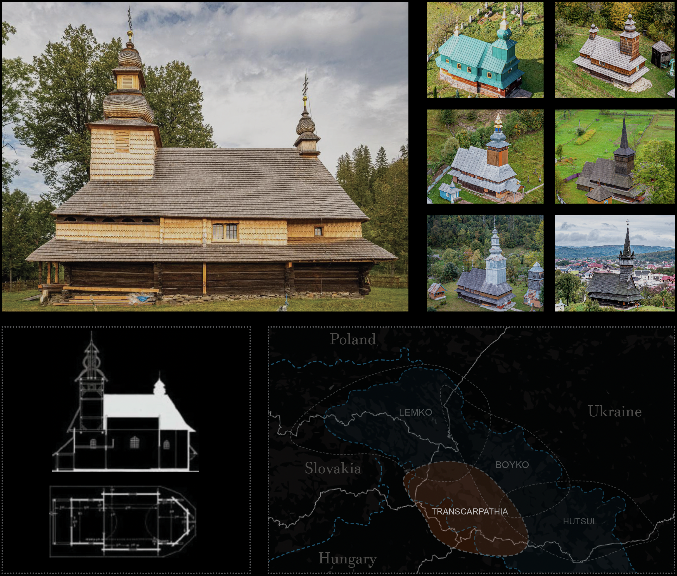
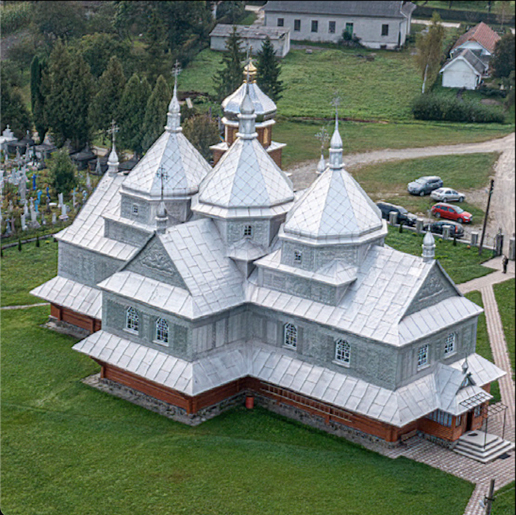
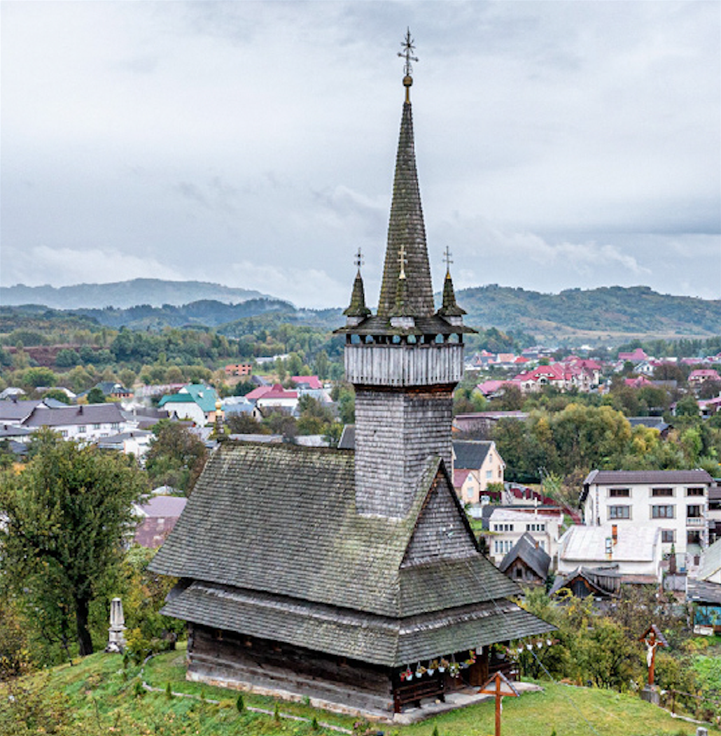
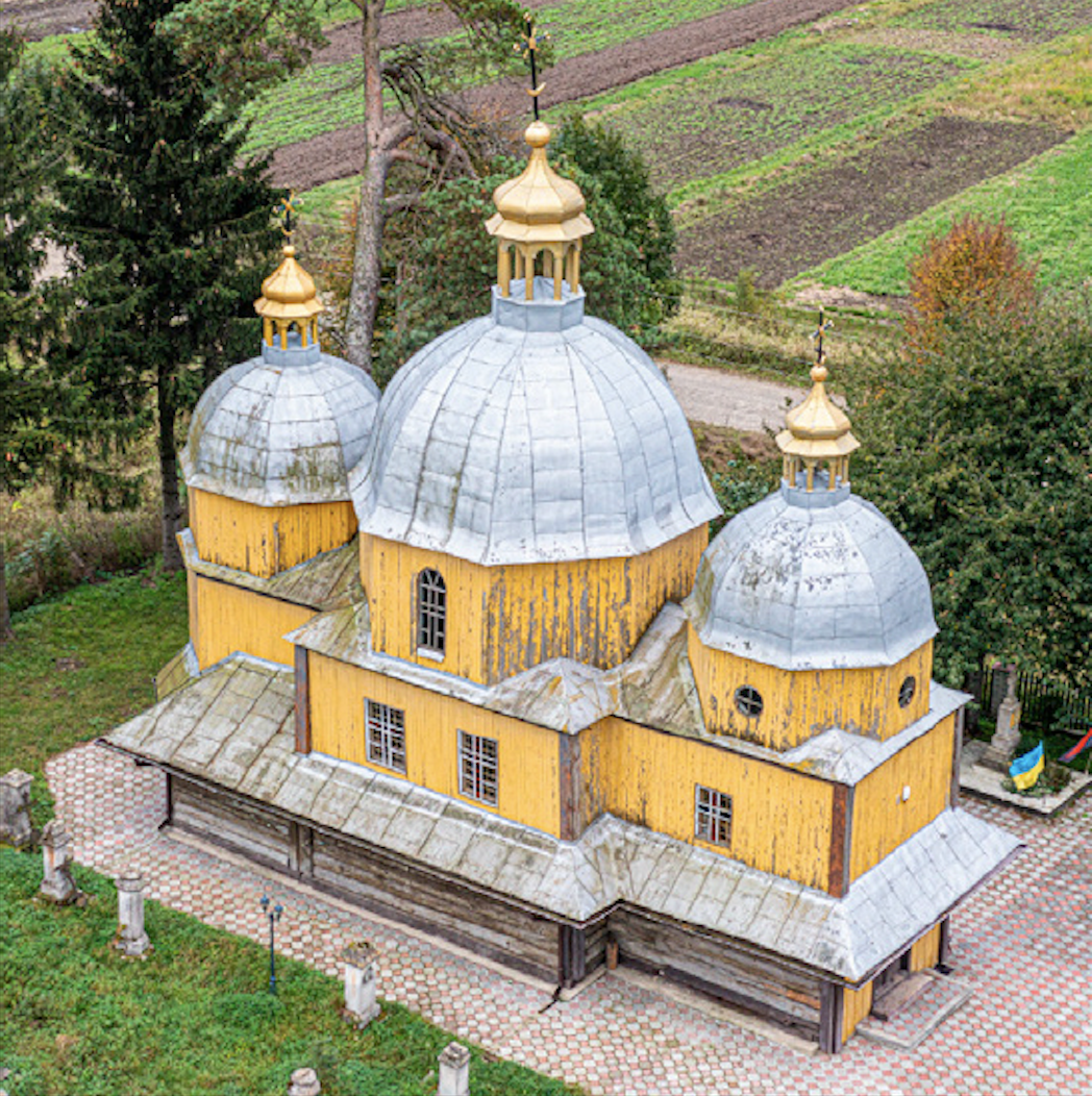
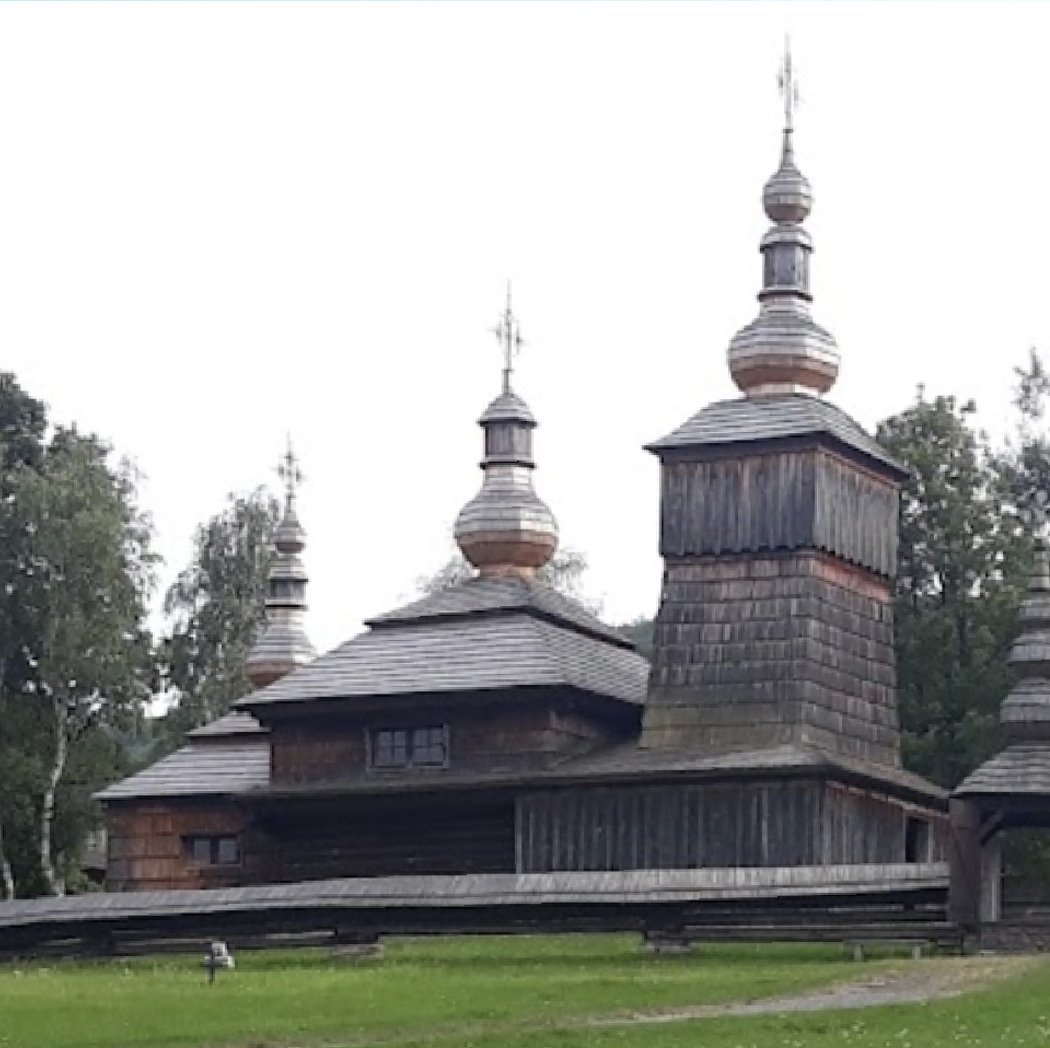
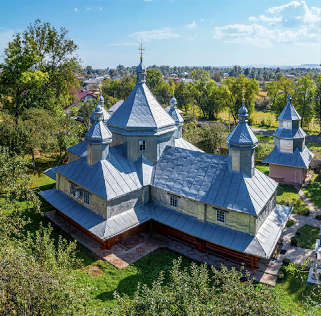
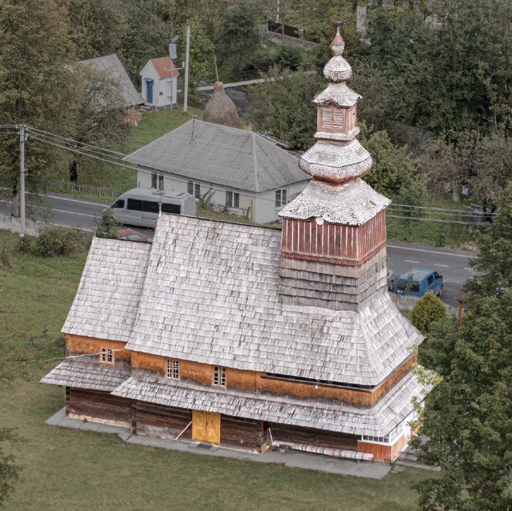
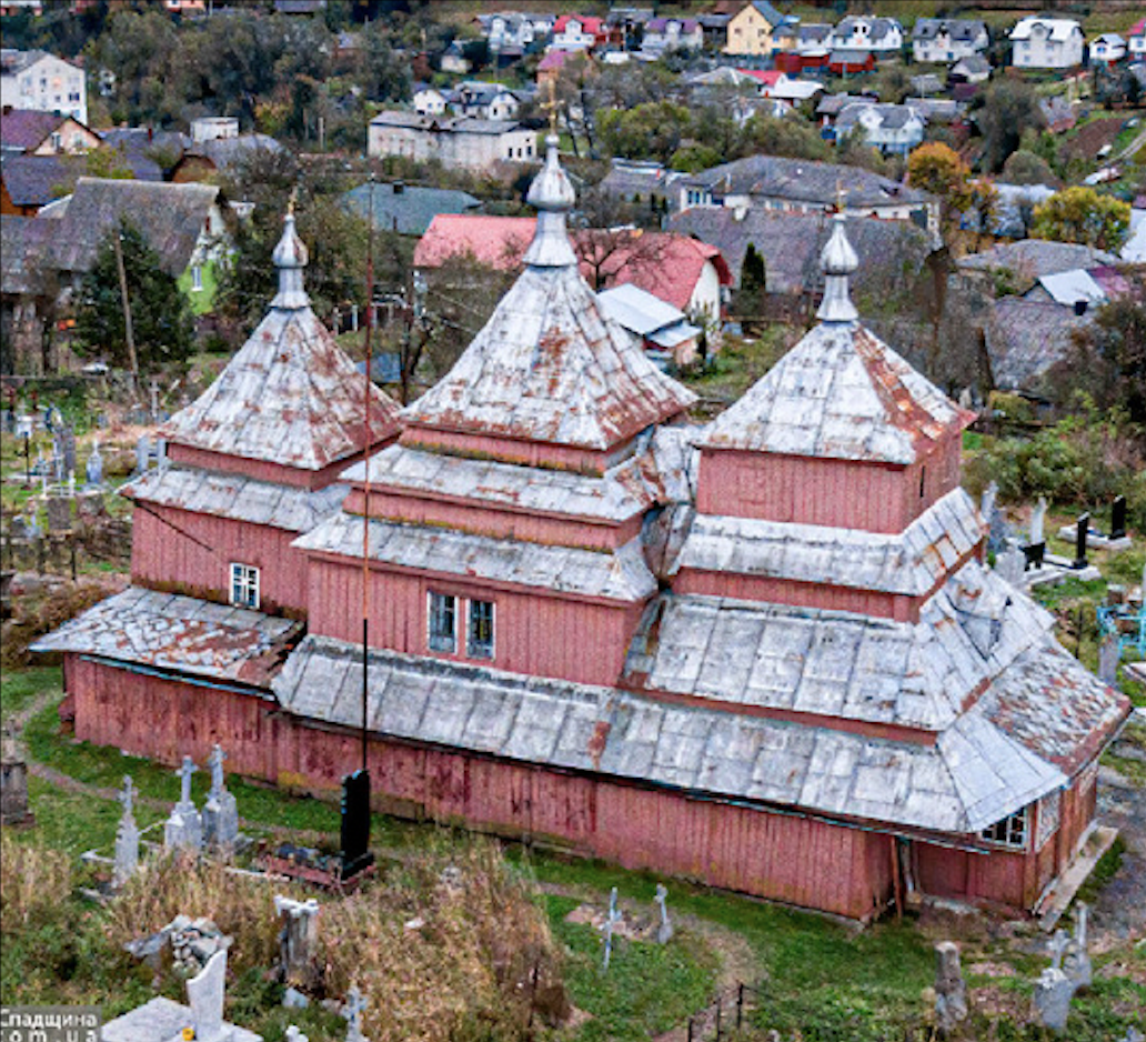
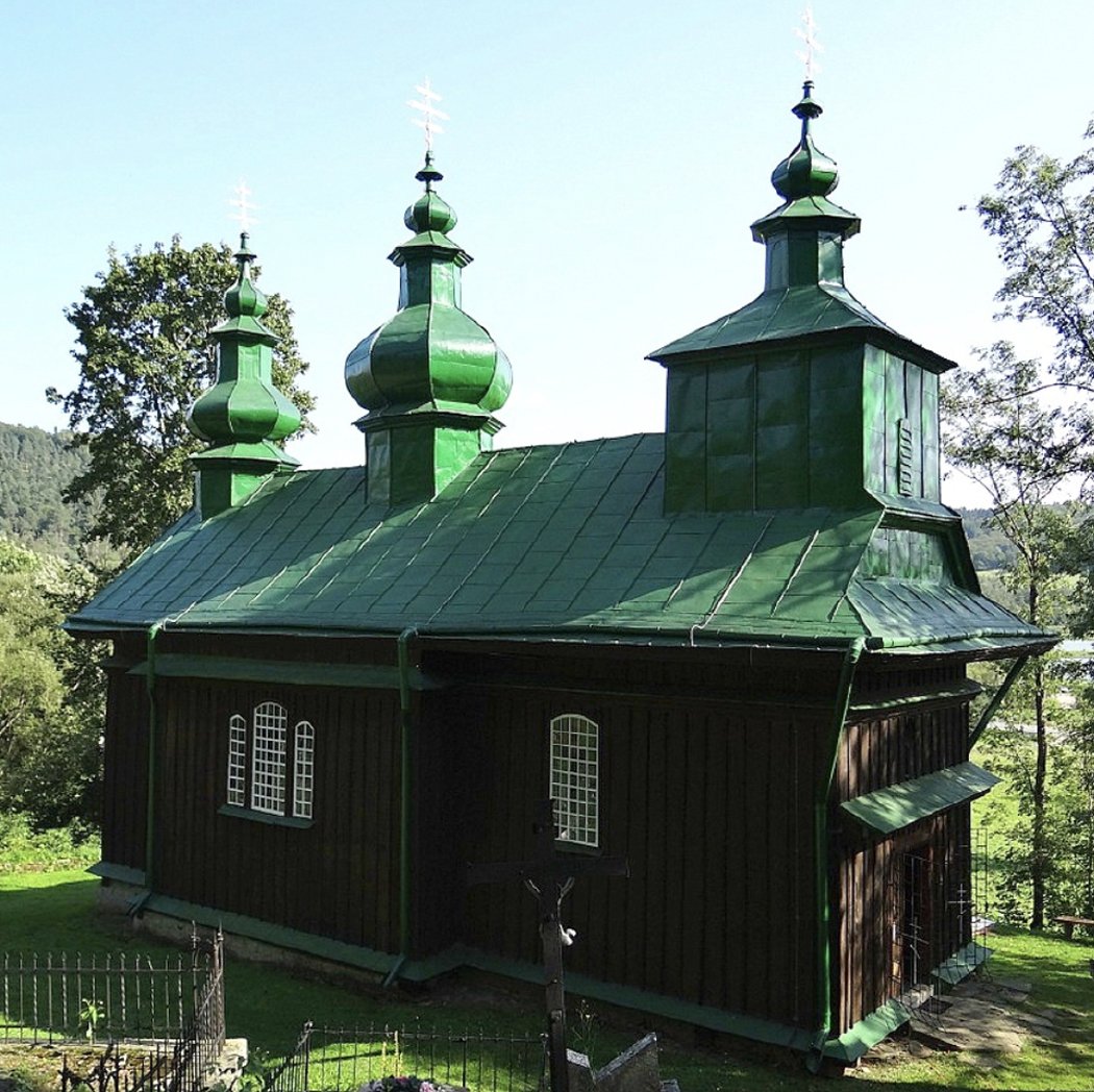
The Wooden Churches of the Carpathian Mountains
The wooden churches of the central Carpathian Mountain region can be generally described as unique examples of a broader, yet long-lost wooden architectural heritage. Unlike their urban counterparts, the rural and historically remote Carpathian wooden churches were subjected to far fewer hazards. For example, risk from fire, vandalism, arson, and replacement with stone architecture which was much more common in more populated urban areas. As such, Carpathian wooden churches pro-vide a unique glimpse into a wooden architectural heritage that has generally disappeared within the rest of Eastern, Central, and Western Europe.
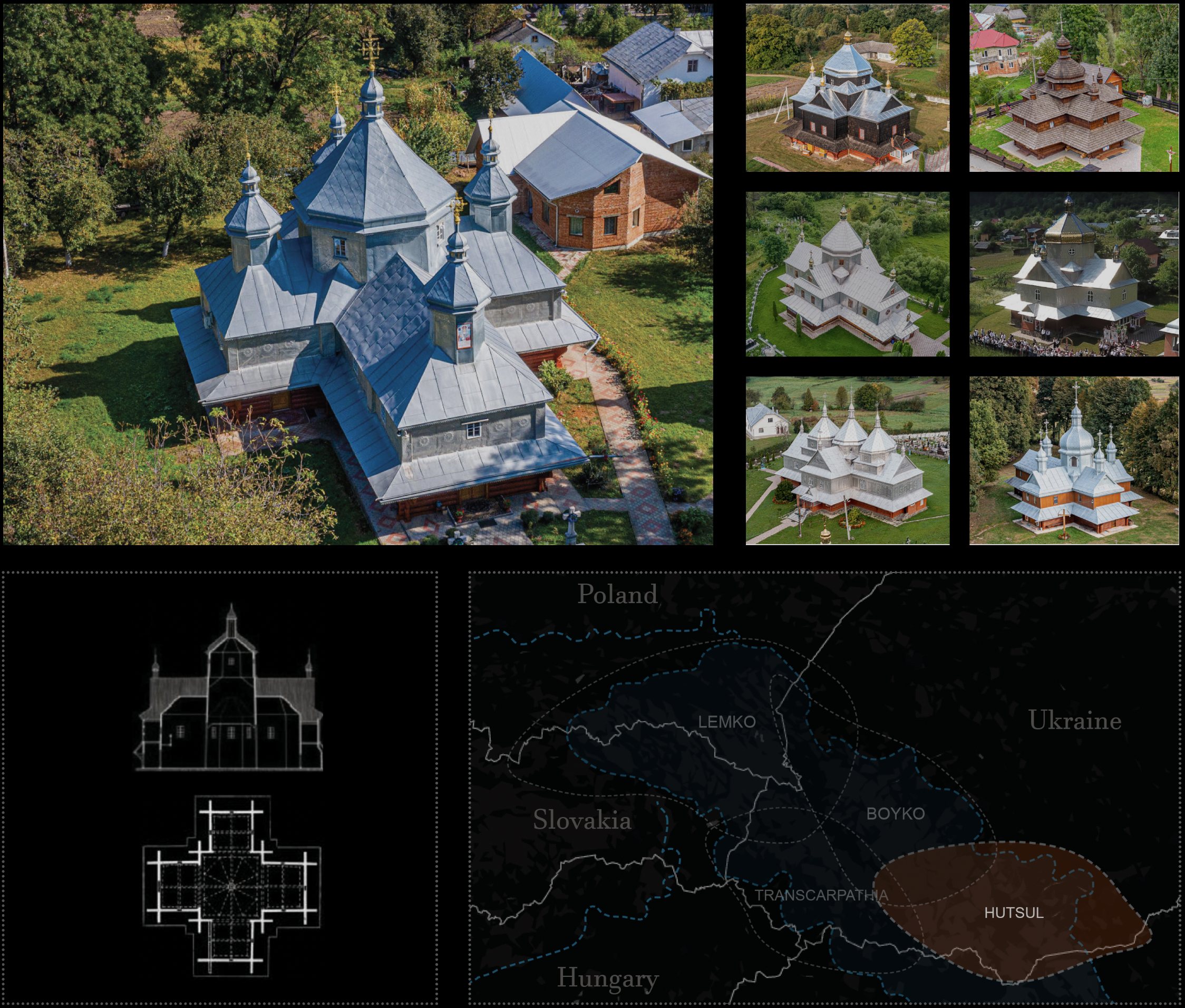
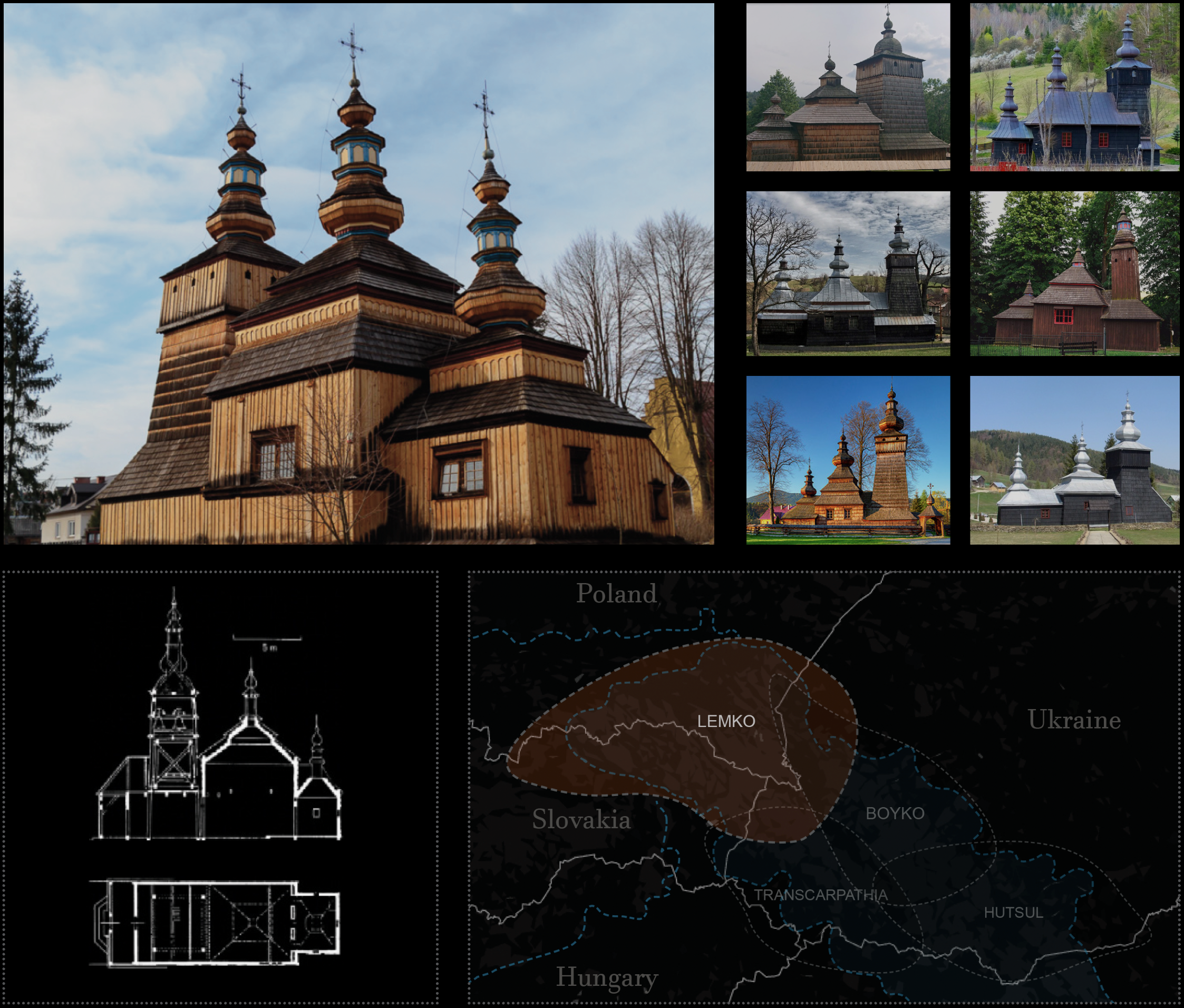
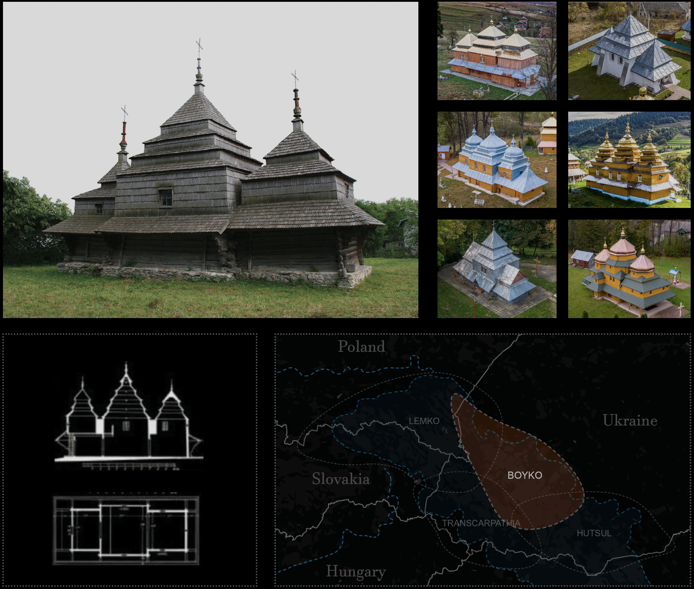
Four Primary Architectural Styles
Boyko, Lemko, Hutstul, and Transcarpathian
To better understand the complex landscape of wooden church morphology from this region, we can generally partition it into four primary styles, or what is commonly referred to as “Schools” of folk temple construction [24]. This include the Boyko, Lemko, Hutsul, and Transcarpathian schools, which are the result of the design inclinations of four distinct cultural groups. In terms of construction date, the vast majority still standing were built between the 18th and 19th centuries, though some are as old as the 17th and even 16th century. Other schools of wooden folk temple construction are also in-cluded in the dataset such as Bukovinia, Pokut, Podilia, Opilska, Przemsyl, Volhynia, Bessarabia. and Transylvanian school though lesser in number. However, the paper will only focus on the main four primary schools represented in our dataset, being the Boyko, Lemko, Hutsul, and Transcarpathian schools.
Process
My process to extract the morphological patterns of churches using deep learning can be partitioned into three broad stages; the dataset construction stage, the DL model training stage, and the model analysis stage. This entire process took 7 months to complete. The dataset construction phase was the most time consuming phase and took 6 months to complete while the model training and model analysis stages were relatively quick and took just over 1 month to complete in total.
Stage 1: Building a Custom 3-D Dataset From Scratch
In order to analyze the 3-D architectural forms of hundreds of wooden churches, we first needed to provide our DL model with, as input, a large dataset of these churches in 3-D, including as many primary and sub-style church variations as possible. Due to the lack of pre-existing digital 3-D data, we used a recently-released computer-vision technique called Neural Reflectance Surfaces (NeRS) to convert just 6-8 digital photographs of a church into an accurate digital 3-D reconstruction. By applying this technique to hundreds of churches, we were able to create our dataset of 313 3-D churches representing various styles from all over the central Carpathian region of Ukraine, Slovakia, Hungary and Poland.
3-D Dataset Creation Process
Constructing a dataset of 3D churches using NeRS and then preparing it for DL analysis requires a nine-stage work-flow (Figure 90): 1) a broad search for churches and acquisition of exterior church images; 2) selection of the final images showcasing all exterior sides of each church; 3) editing the images to remove occlusions, correct perspective distortions, and compensate for missing images; 4) creating image masks representing the location and outline of the church; 5) estimating image angles between the camera and the church; 6) estimating the general dimensions of the churches (length, width, and height) ; 7) reconstructing a high-quality detailed 3D mesh object, 8) Augmenting the data from 331 churches to 5627 models, 9) converting the models to SDF voxel format.
Step 1: Searching for Churches & Collecting Imagery
The wooden churches used in this research reside within the mountainous, foothill and water-shed region of the Carpathian Mountain region of Central Europe. In order to build the dataset, digital images of over 400 churches were manually searched for and collected over a one month period. In total, over 10,000 images were collected, representing 409 unique churches from the central Carpathian Mountain region showcasing a wide range of distinct styles and sub-styles. Images were acquired from a number of online resoures, including, but not limited to, Google Earth, various academics and domain experts, various blogs, and multiple image repositories that specialize in historic architecture of this region.
10,000+ images collected

Step 2: Image Pre-Processing
Images for each church needed to be carefully pre-processed and prepared for 3-D reconstruction. First, the final images required for the 3D reconstruction process need to be selected. Then, some images were altered in order to ensure their associated church was accurately reconstructed in 3D. For example, images occasionally had to be manually edited or constructed to provide the front or rear elevations. Next, object masks needed to be provided for each individual image. Then, both the horizontal and vertical camera angle between the camera and the church for each image was manually recorded to a JSON file. Next, a custom script was created to automatically duplicate images and horizontally flip them to represent the other side of the building. Finally, the dimensions of a shape template corresponding to the estimated approximate size of each church must be determined
Step 3: Reconstructing Churches in 3-D
Once all images have been preprocessed and their corresponding JSON files complete, the final stage of the reconstruction pipeline (Figure 113) was reached and each church was reconstructed from the images as a high-quality detailed mesh object using the NeRS algorithm. To reconstruct each church a remote computing cluster containing 4 GPUs (NVidia GeForce GTX Titan X with 12 GB of VRAM) was used to expedite this process. Once completed, the reconstruction quality of each church was manually inspected. Out of the original 409 churches, 96 could not be recon-structed due to insufficient imagery.
Church Reconstruction Examples
Final 3-D Reconstructions
The dataset of reconstructed churches includes 313 individual buildings (Figure 115, 116). The dataset were then automatically augmented from 313 buildings to 5,627 buildings using an algorithm that made slightly different copies of each building through a series of random rotation and scaling transformations.
313 Reconstructions
Augumenting the dataset from 313 to 5,627 churches in order to adequately train our VAE model.
Step 4: Augment Dataset using Synthetic Data
In order to sufficiently train the DL network and extract a reasonable latent space distribution, where latent space is a representation of abstracted data where similar data points are clustered closer to-gether, the dataset needed to be augmented from 313 buildings to 5,627 buildings. Data augmenta-tion is common technique if the dataset is insufficiently large to train a DL-model and helps prevent overfitting [32]. Overfitting is when a model begins to memorize hyper-specific features of the data, rather than more useful general features of the data that might help better describe it as a whole. To avoid overfitting, the dataset was augmented to be 17X its original size by making 17 copies of each building, with each copy being slightly different from the next through a series of transformations such as rotation and randomly scaling. To expedite this process, a custom script and data pipeline was created in Grasshopper, a parametric design software used to create and manipulate 3D geometry.
Stage 2: Model Training
In order to analyze the 3-D form of our 5,627 building dataset, we use a subset of Artificial Intelligence called Deep Learning (DL), which is an algorithmic method used to extract complex statistic-based patterns from large collections of data. For this research, our DL network “learns” the range of church styles in our dataset by analyzing thousands of examples at a time in order to find reoccuring data patterns. For instance, re-occuring church styles such as Lemko or Boyko style. Then, by encoding these style patterns as unique sets of 128 numeric values, where each value represents a particular feature of that style, for instance bell-tower height, they can then be compared to one another according to the similarity or differences of these numbers.
Compared to more traditional methods, which take time, are often manual, and can analyze just a handful of buildings at once, these new statistic-based techniques can be applied to analyze the styles of thousands or even millions of buildings at a time. And after a relatively short processing period, provide the means to explore and identify both complex and difficult or impossible to detect morphological patterns that permeate through very large collections of buildings or other urban data.
Step 1: Model Selection
The neural network architecture chosen for form analysis is a variational autoencoder (VAE). Generally, VAE consists of two neural networks, the encoder (E), which converts input data into an encoded rep-resentation (Z), and the decoder (D) which reconstructs the data from the encoded representation. Together, VAE aims to “jointly [learn] deep latent-variable models and corresponding inference models using stochastic gradient descent”. In other words, they aim to fit a probability distribution to the features of the data. When reconstructing these data features, there is a loss score which, in general, is the difference between the original and the reconstructed data. This loss score is then used to update the parameters of the distribution to better fit, or match the original data features, thus decreasing the loss.
Step 2: Model Training
Training was carried out using a VAE model for 3000 epochs over a period of just over 4 hours. To adequately tune the model, the following hyper parameters were used: a batch size of 32, a single learning rate of 0.00005 with Adam optimizer, and a latent space size of 128. Data was split into a 5,065-object training set and 562 object test set using a standard 1:9 ratio. At approximately 330 epochs, the training and test errors intersected leading to slight overfitting and a final train - test error difference of 0.02. The final training loss was 0.34 and the final test loss was 0.32 suggesting only negligible overfitting (Figure 125). Convergence occurred just after 900 epochs. Reconstruction of the encoded data is show in Figure 126 and displays satisfactory results.
Stage 3: Model Analysis
Once training was completed and the model could satisfactorily encode and decode the dataset, both statistic and heuristic-based techniques were used to identify both macro and micro architectural form patterns learned by the model. DL-based analytical techniques include clustering churches according to similar form and determining typical and least typical forms within cluster, while heuristic techniques include references to geographic distribution data and the findings of past research.
Some patterns identified include; how tower height and placement were the most significant architectural indicators of specific church styles within this region and how church-types morph from one style into the other over geographic space. By combinding both DL and traditional techniques, complex form patterns, which were difficult or impossible to identify using human cognition alone, can now be identified, discovered, and revealed amongst hundreds of churches at a time.
Describing Building Forms Using 128 Numbers
The power of Deep Learning (DL) resides in its ability to extract the foundational rules and patterns that govern extremely complex data and then abstract these rules into simplified and easy-to-interpret representations. In this way, complex phenomena, such as historic weather patterns or the typical DNA sequences of particular populations, that may be impossible to describe using human cognition alone can now be unravelled and easily described using DL.
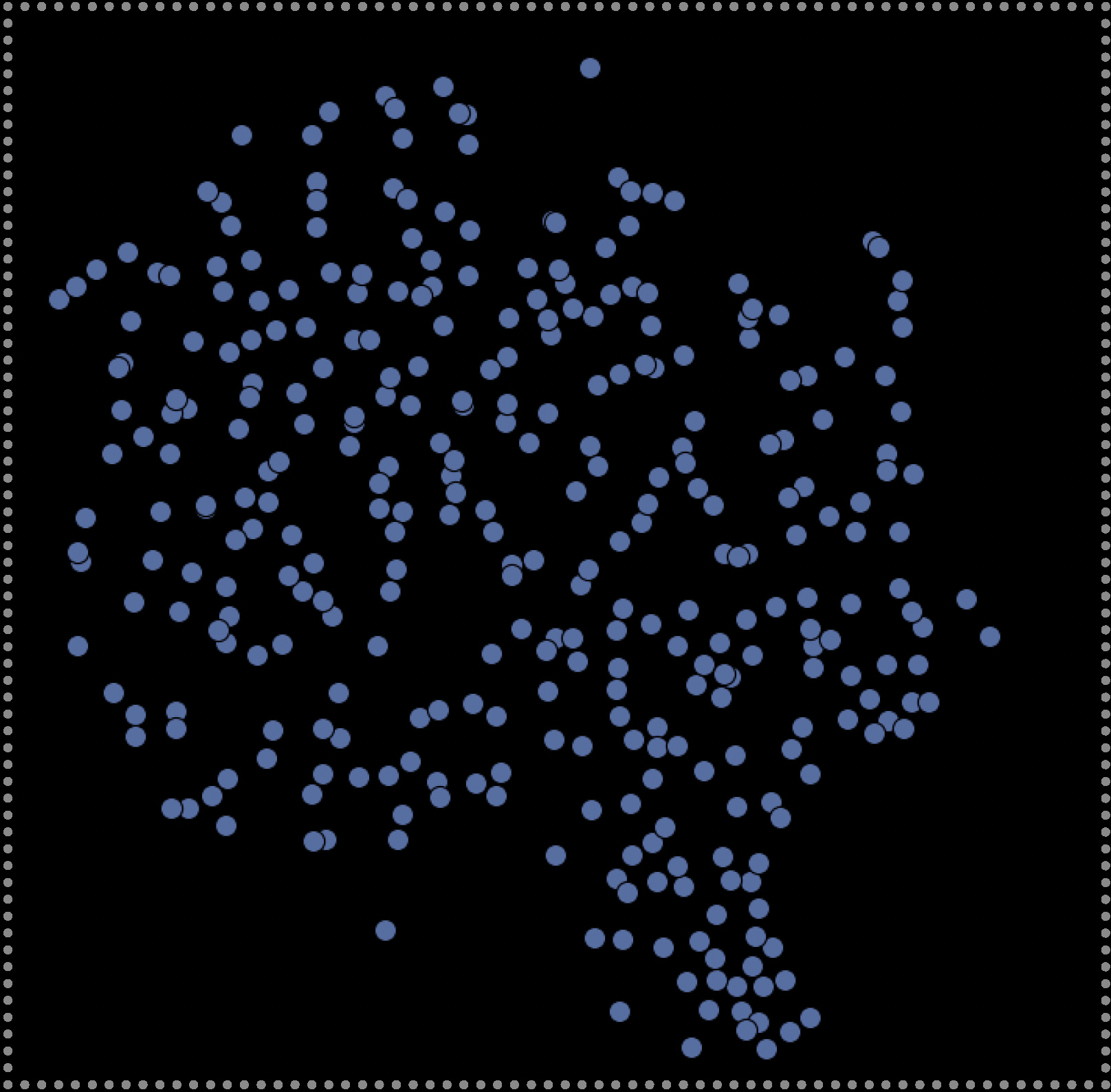
In the case of architectural form, DL models have the ability to extract both the nuanced and complex rules and geometric parameters that define the forms of hundreds, thousands or millions of buildings at a time. In this research, the rules that define church forms are encoded as 128 unique numbers, with each number quantitatively describing one morphological aspect of that building such as building height. This formulaic method of architectural quantification allows us to compare one building to another using these 128 numbers. In order to visualize these relationships, we can abstract these numbers into just 3 in order to represent each building in 3 dimensional space as shown to the right. Here, each point represents a single church with proximity between church points indicating their level of form similarity. While points closer together indicate increased form similarity, points further apart indicate less similarity. From this, we can then extrapolate that points clustered tightly together may indicate particular building styles. For instance, churches with three equal height towers, or churches that have a cruciform layout. By color coding these tight groups, we can better visualize and explore these potential style groups. By changing cluster size, we can explore both broadly shared overarching styles shared by hundreds of buildings or hyper-specific micro-styles shared amongst just two or three buildings.
Step 1: Visualizing our Learned Data
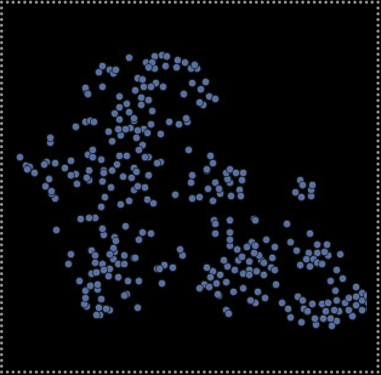
To visualize and determine what was learned by our model, we clustering churches according to similar morphology, which here are represented by their unique z-values (Rhee 2019). To begin this process, each original church needed to be individually transformed into its 128 latent-vector representation, or more commonly referred to as its “z-value”. These z-values can be obtained by encoding each 3D church with the pre-trained VAE model as described in the previous step. However, as the dimensionality of these z-values is too high to visualize (128 dimensions), they must be abstracted and reduced to just two dimensions. To do this, t-Distributed Stochastic Neighbour Embedding (t-SNE) [59] was used to reduce high-dimensional values, 128 in this case, to low dimensional representations, two in this case, while preserving as much of the original data distribution as possible. This is done to increase interpretability and allow us to visualize complex, multi-dimensional data. When each of the 313 z-values are converted to just two dimensions (an x and y value) then displayed on a scatter plot, their position from one another within the plot represents their degree of morphological similarity. Thus, points that are closer together indicate church forms with increased similarity and ones that are far apart indicate church forms with less similarity. In this way, we can visually see and understand church’s morphological relationship to all other churches within the dataset.
Step 2: Choosing a Latent Space Representation
By testing different T-SNE parameter settings, various latent space representations were explored with the final one chosen due to its well partitioned data configuration. For example, by iteratively testing different T-SNE parameters and surveying results, we determined which values increased cluster interpretability according to our understanding of church forms informed by existing research and expert knowledge. Though this process influenced our results, it enhanced our ability to identify and analyze patterns that could have otherwise been missed.
For this paper, I used the following t-SNE parameters to reduce the dimensionality of the datasets latent-vectors from 128 to 2. Number of components was set to 2, while perplexity, learning rate, and number of iterations remained at the default values of 30, 200 and 1000 respectively.
Step 3: Clustering Latent Space
Identifying both complex and subtle clusters among hundreds or thousands of individual z-value points can be a challenging, if not impossible task dependent on the size and complexity of the dataset. To assist with this task, I used a technique called “Density-Based Spatial Clustering of Application with Noise” (DBSCAN) [60] which searches for and color codes clusters according to point density. Search parameters can be controlled by setting DBSCAN hyper-parameters such as the “minimum number of samples” (mns) in a neighborhood for a point to be considered a “Core point” of a cluster, and “epsilon” (eps) or the maximum distance between points to be considered as being within the same cluster neighborhood. In this way, clusters can be more easily discovered, explored and identified via color coding to reveal both large clusters representing broader church form similarities and smaller clusters that may indicate more niche or narrowly shared form characteristics.
Clustering latent space according to loose, large-sized clusters (left), medium-sized clusters (middle), and small tightly-grouped clusters (right). Gray points represent churches with outlier forms that cannot be easily grouped due to insufficient numbers of similar examples, or by less frequently, geometric distortions due to reconstruction errors.
Step 4: Defining Cluster Evaluation Techniques
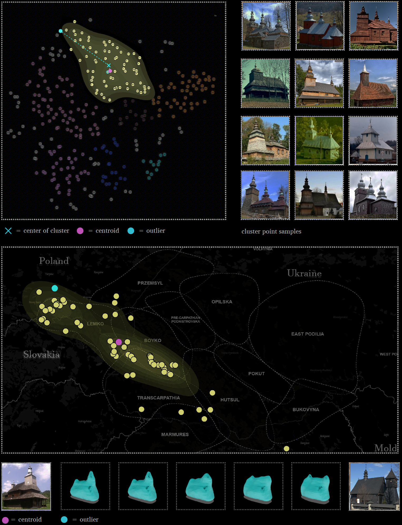
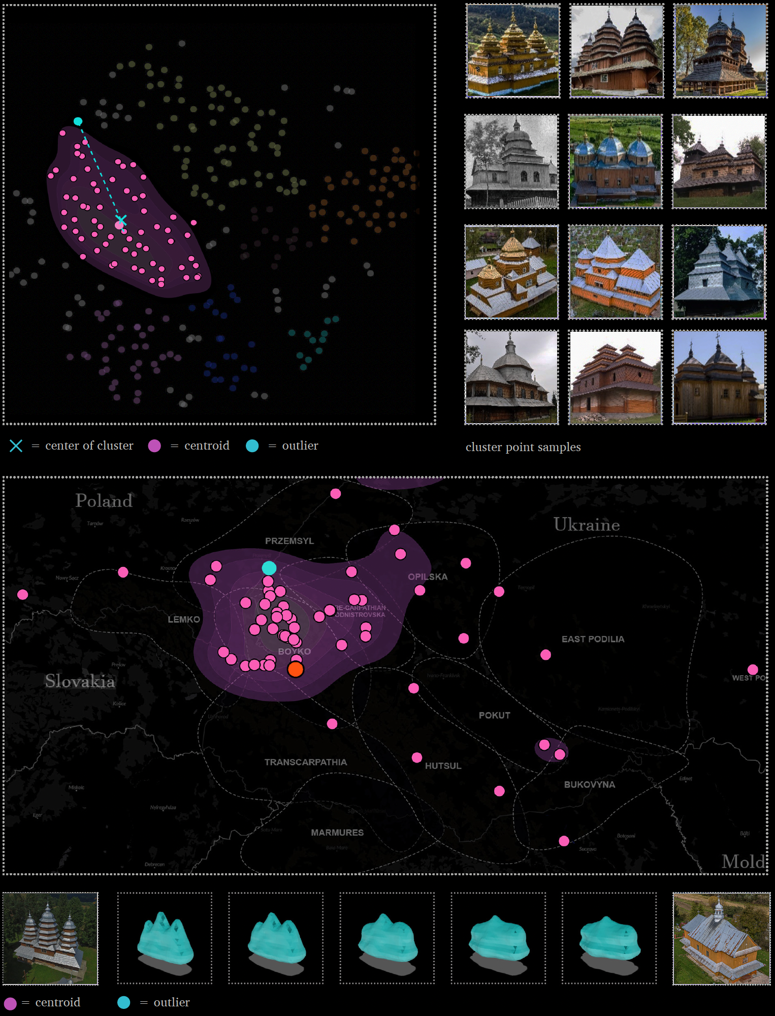
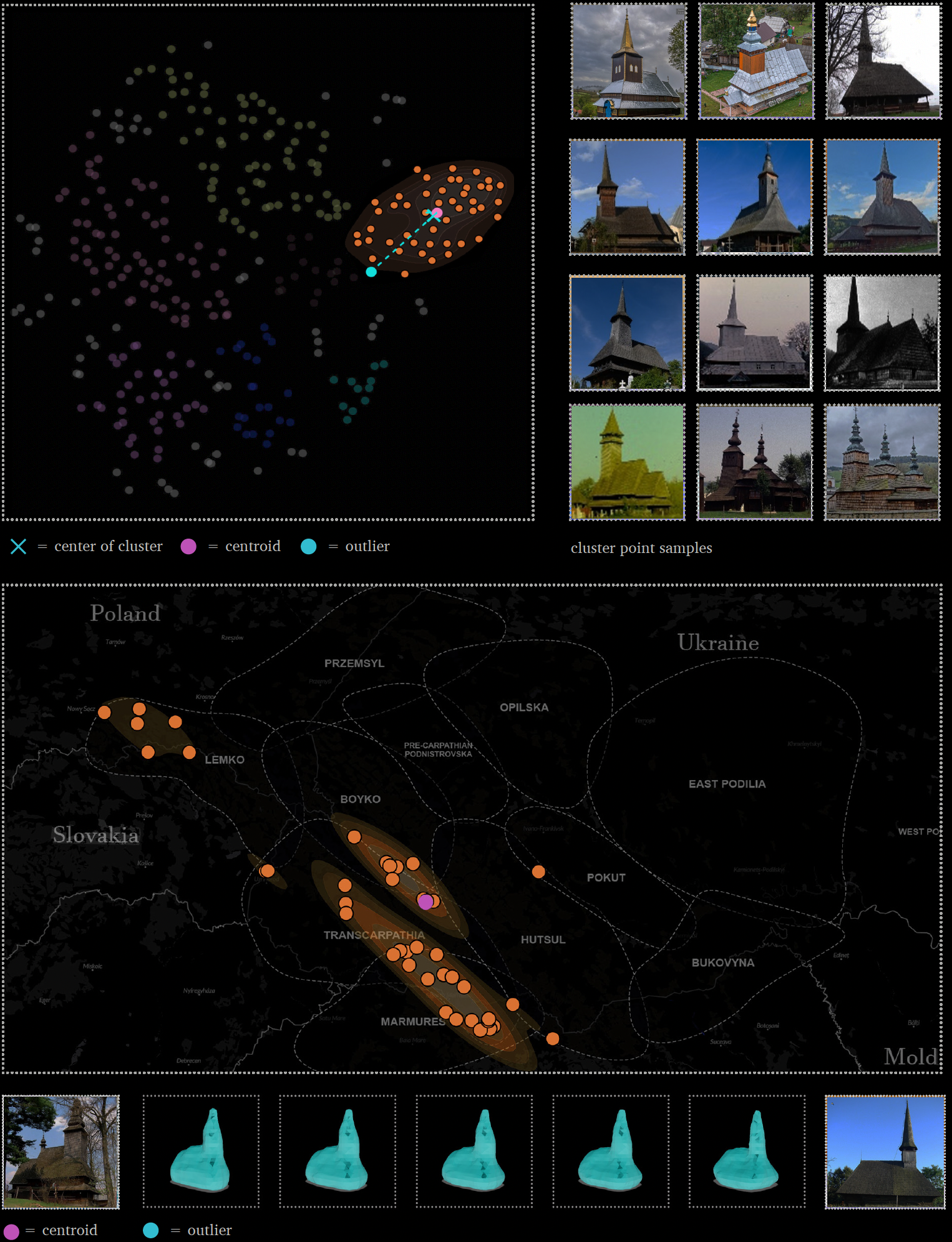
To better understand and interpret the morphological significance of and patterns within each church cluster, we evaluat-ed them using three different methods. First, by cross checking each cluster of churches against existing research. Secondly, by analysis of and visual interpolation between cluster centroid and periphery data. Thirdly, by mapping each cluster to geographic space and comparing against agreed upon cultural zoning information.
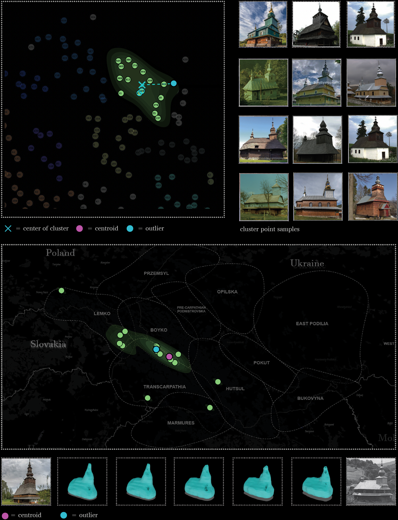
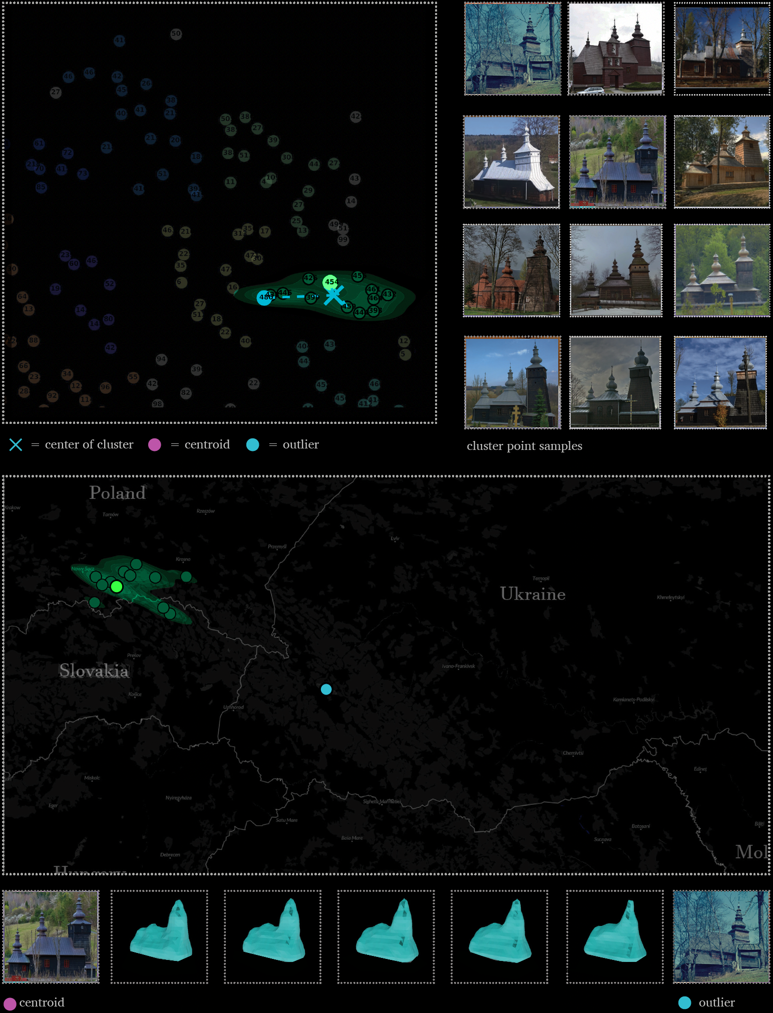
Method 1: Cluster Centroid & Outlier Analysis
The third method (Rhee 2019) provides further cluster analysis by sampling the nearest church point to the centroid of the cluster. As clusters are identified by t-SNE and propagated outwards from a central dense core cluster, it can be understood that the centroid represents the “typical” or “average” church form of that cluster. This provided me with the means to retrieve the “typical form” of each cluster, thus identifying the general morphology represented within the given cluster. Equivalently, defining the furthest church from the centroid and interpolating (morphing) between the two in 3D model space, via an interpolation animation video, helps to visually see the range of morphological variation within the cluster. A custom algorithm was built to determine both the centroid church and furthest outlier church.
Method 2 : Form Comparison with Existing Research
To evaluate the clustering results, we cross-checked the results against existing materials, such as church style diagrams from existing research, reference to the original 3d models, and domain knowledge gained from discussion with experts. Through this crosscheck, we confirmed that particular church styles were being grouped together within the clusters. For example, churches with a single tall tower suggesting the Transcarpathian school of design, or churches with three low towers suggesting the Boyko school of design. In particular, Yaroslav Taras’s 2020 publication “Wooden Temple Architecture of the Ukrainian Carpathians” was considered a significant ground truth benchmark for comparison as it, to the best of the authors knowledge, represents the most current, extensive, and detailed description of the Carpathian wooden churches, and their complex and interrelated styles and sub-styles
Method 3: Geographic Distribution Comparison with Existing Research
For the second method, we mapped each point in the cluster to geographic-space and compared their distribution to existing research that defined the architectural-ethnic boundaries of the various styles and sub-styles of these churches. In this way, we investigated which regional style(s) or sub-style(s) the cluster might represent by visualizing the geographic position of all churches within that cluster (Figure 131). However, as architectural-ethnic boundaries overlap, and unique church styles from one cultural region can be found deep within another, resultant observations using this final method should be considered suggestive rather than prescriptive. Yaroslav Taras’s 2020 publication “Wooden Temple Architec-ture of the Ukrainian Carpathians” [25] was used as a ground truth benchmark for geographic comparison and reflection.
Diagram showing the analysis of a micro cluster using method 1 (left side - form comparison) and method 2 (right side - geographic distribution comparison)
Step 5: Reviewing Clusters
By using the three methods of cluster analysis, I was able to review each cluster according to its architectural characteristics, typical and least typical forms, geographic dispersion, and relation to real church style categories identified by previous research. In this manner, I was able to determine how broad or specific each cluster was in terms of grouping churches together according to shared form characteristics. For this research, three various clustering configurations were investigated:
Large Low-Density Clusters
Contains churches that shared general overall architectural characteristics.
As a result, various sub-styles are clustered together
Geographically, churches within these clusters are more loosely spread
Medium Sized Clusters
Contains churches that contain more specific shared architectural characteristics
Contains fewer sub-styles as it is more specific
Geographically, churches in this cluster are more concentrated
Small High-Density Clusters
Contains churches that shared general overall characteristics.
As a result, various sub-styles are clustered together
Step 6: Comparing Clusters Against Ground Truth Labels
By referring existing research, ground truth (G.T.) style labels were applied to each church point in our 2D latent space scatter plot. These labels indicate which School of folk temple construction they actually belong to in reality. By having these labels, I was able to better evaluate how well our model was able to cluster capture the primary morphological traits of these primary style groups. When referring to the latent space diagrams, it is clear that there is correlation between the G.T. labels and the original clusters predicted by the model.
Findings: Macro & Micro Form Patterns
By applying statistic and heuristic-based techniques, both macro and micro architectural form patterns were identified amongst the latent space data distribution. While macro patterns help to explain the overall morphological organization of the latent space, micro patterns help reveal how smaller sections of the latent space are distributed. In turn, they both reveal the architectural features that are most broadly and most narrowly shared amongst the churches within the dataset. The following section illustrates and discusses these findings and their contribution towards our overall understanding of Carpathian Wooden Churches and their complex form relationships to one another.
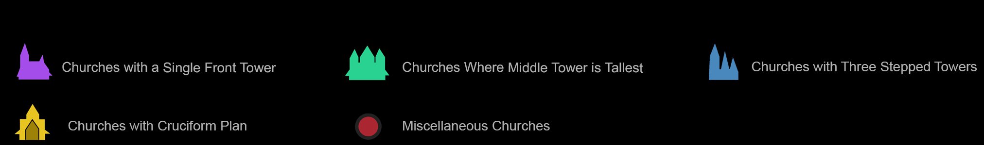
Macro Pattern 1: Front Towers vs Middle Towers
The first macro pattern identified partitions the entire latent space distribution in half diagonally from the extreme top left to the extreme bottom right. The right half, includes churches that almost always have its tallest (and usually only) tower located at the front of the church over the narthex. The left half, includes churches that almost always have its tallest tower over the center of the building above the nave. Though some churches on the left side of this dividing line are towerless, they almost always have a stepped hip-roof configuration with the highest hip roof in the middle over the nave, and two lower step hip roofs of equal hight on eitherside over the narthex and sanctuary. This demonstrates how all churches with-in the dataset as well as their associated styles and forms can be generally organized, identified, and related to one another according to tower height and placement.
Macro Pattern 2: Church Form Distribution
The second macro pattern identified is the general partitioning of latent space into four zones according to different ar-chitectural form characteristics: Zone 1 includes churches with one tower over the narthex at the front. Zone 2 includes churches with three towers with the tallest over the Narthex at the front. Zone 3 includes churches with the tallest tower over the Nave in the middle. Zone 4 includes churches that have cruciform floor plans.
Macro Pattern 3: Tower Height & Count Changes
The third macro pattern identified is the change in tower height and number of towers present. This particular macro pattern occurs in multiple directions across the latent space, indicated by the red arrows in the figure. By finding and illus-trating this trend, I obtained a deeper understanding of the dataset by providing a means to compare the tower height and count of one church to the next. It is also clear that this pattern does not occur in a single linear direction, but rather in a complex multi-directional manner across the latent distribution diagram. This complexity makes it difficult to both detect and track without careful study of each cluster and an intimate knowledge of the subject through domain knowledge and experts and reference to existing research and geographic space.

Micro Pattern 1: Lemko Church Form Transition
The image below illustrates the first micro trend; how the form of Lemko churches morphs across the latent and geographic space in terms of tower height and size. The transformation occurs from left to right within a medium sized cluster near the center of the distribution, partitioning three smaller clusters based on a particular height and size of tower: the cluster in purple includes churches with the shortest towers; the cluster in red includes medium sized and height towers; the cluster in green includes the largest and tallest towers. These three clusters were then compared to Taras’s sub-style diagrams, and somewhat align with three distinct Lemko sub-styles. The shortest (purple dots) are associated with the North (with towers) sub-style, the medium (red dots) with both South (Slovak) and Northwest Late sub-styles, and the tallest (green dots) associated by primarily Northwest Late sub-styles. By identifying this pattern, we can understand how both tower height and size are important architectural characteristics that help define or relate particular Lemko church sub-styles to one another.
Micro Pattern 2: Boyko to Lemko Style Transition
The below figure illustrates the morphometric relationships between the Classic Boyko sub-style and the Northwest Late Lemko sub-style churches, and how their forms morph from one to the other, as represented by a series of transitory intermediate, or hybrid styles, across latent space. This transformation occurs along a curving path from left to right as indicated by the blue arrow below with the Classic Boyko sub-style (red dot) churches loosely clustered around the left-middle side of the distribution and Northwest Late Lemko sub-style churches (blue dot) tightly clustered within the middle. As you move between the two points in latent space from left to right, we encounter various church styles which appear to be represent transitionary stages between these two distinct styles. Overall, this pattern illustrates how our model could linearly organize this transition between Boyko and Lemko style within latent space. Furthermore, when plotting these patterns to geographic space, this transition also appears to follow a linear pattern as well with the most noticeable hybrid styles occurring in the border regions between both cultural zones, suggesting how style gradually transitions over space.
Micro Pattern 3: Transcarpathian to Lemko Style Transition
Another micro-pattern identified demonstrates the relationship between Transcarpathian Marmures regional style (red dots) and Lemko style (greend dots), and how they transition from one to the other. In latent space, both styles are found within their own clusters at the right side of the distribution, with the Marmures churches at far right and the Lemko cluster to its left. Points in between represent a mixture of various Transcarpathian sub-styles. However, their proximity to one or the other determines the their level of morphological similarity to either the Marmures or Lemko style. For example, points closer to the Lemko cluster begin to express Lemko-like features, like additional towers or lower sanctuary rooflines. Similarily, points closer to the Marmures cluster begin to reflect their signature taller towers and continues rooflines over the nave and narthex. In map space this is reflected geographically in a Northwest direction beginning at the Marmures region at the bottom right corner and ending in Lemko region in the top left corner. The order of points in-between also generally correlatesto their order in latent space, suggesting how style transitions occur incrementally over geographic space as well.
Micro Pattern 4: River & Valley Micro Styles
A conversation with Mykhailo Syrokhman revealed that certain church sub-styles can only be found within certain valleys or along short stretches of rivers. In order to identify these micro-style using DL-methods, the latent space distribution was re-clustered in a way that only highlighted the smallest and most tightly grouped church points. As a result, two clusters were detected: a small cluster of two Boyko churches within a single valley (Figure 179) and a group of three Transcar-pathian School churches along the same stretch of river (Figure 180). Both built during the 18th century and located only four kilometers apart, these two Boyko churches appear almost identical and embody a unique Boyko sub-style possibly endemic to that specific secluded region.
The three Transcarpathian churches have two neighboring latent space tertiary-clusters. They are located in close proximity to one another along a short stretch of the Latorica river within the northern Transcarpathian zone. The churches were built around the early 19th century. They are almost identical, but do not appear to fall within a described sub-style category, suggesting the presence of a unique micro-style within that region repre-sented by just a few examples. Finding these groups highlights how DL-methods can assist us with identifying multiple unique micro-styles relatively easily amongst datasets of hun-dreds or tens of thousands of examples.
Micro Pattern 5: Tripartite to Cruciform Plan Transition
Another noticeable form pattern indicated by the purple arrow is the transition from tripartite to cruciform plan which occurs between the bottom of zone 3 and zone 4 (Figure 181). Though the typical form of zone 3 is mainly represented by a linear-tripartite plan, it does start to transition towards a cruciform plan at the bottom as it nears zone 4 (church 1). This is marked by churches that have increasingly wider nave spaces which in turn, begin to give the church a noticeable cruciform shape (church 2). With churches nearer to zone 4, these projections tend to get larger, hence increasing this cru-ciform effect. Once in zone four, the most pronounced cruciform shape is present (church 3). From these observations, we can assume that as churches within zone 3, represented as points, approach the border with zone 4, they may increasingly express a cruciform plan configuration, with the most pronounced configurations being found deep within zone 4.

Micro Pattern 6: Border Styles
An additional micro trend revealed three churches that appeared to be nearly identical though they are part of only two dif-ferent primary style groups: Lemko Snynskyi sub-style (#1, 2) and Transcarpathian Velikobereznyansky-Chor-nogolovska sub-style (#3). In latent space, all three churches are close together, hence suggesting similar form and possible architectural-cultural relationship. However, we can see that the model correctly placed both Lemko Snynskyi sub-style churches close together in latent space within the same micro-cluster due to their nearly exact same style. Furthermore, church 3 was plotted further away and within a different, though neighboring cluster due to both its slight differences and overlapping features. When plotting them to geographic space, they appear noticeably close together, suggesting potential cultural overlap. Though morphologically similar, closer inspection revealed subtle differences including differing front facades, roof shapes, and bell tower geometries. Interestingly, all three churches are located within close proximity to each other and right around the border of both the Lemko and Transcarpathian style regions. Their similar form may be the result of the cultural overlap and blurring that occurs at these ethnic boundary zones. Based on this micro trend, churches in these regions could be classified in a new way, such as being a “border style” which can fall within multiple primary style groups at once.
Findings: Misleading Clusters, Patterns & Outlier Churches
While analyzing the latent space distribution, a number of strange clusters were identified that appeared to contain unusual and seemingly unrelated collections of churches. Upon further investigation, it was determined that our DL model was grouping churches by strange architectural features that had little to do with particular cultural styles and more so to do with miscellaneous or less-meaningful geometric forms. For instance, large boxy building additions or flat roofs, which occasionally occurs amongst all church styles. Additionally, poorly encoded outlier church styles which are represented by just few examples also tended to get clustered together within highly style-variable groups. In combination, these observations highlight how DL-based findings should not be taken for granted, may be misleading , and can lead to innaccurate results if not carefully reviewed beforehand and corroborated with domain knowledge and the findings of previous research.
Misleading Cluster 1: “T” Configuration Church Cluster
An unusual cluster includes a large group of churches that at first glance only seemed tangentially related by their hip roof configurations and minimal planar exterior walls. More noticeable were their differences, being a seemingly random collection of churches of different styles. Nevertheless, latent space suggested they were very similar given their densely latent space grouping. After investigating, it was suspected that the clustering may have been caused by the presence of noticeable building additions added to both sides of the backs of these churches. These later addi-tions gave the churches a “T” configuration, which for all schools of temple is highly unusual. However, the model appeared to have considered this unusual characteristic as an important “defining” feature, thus leading to the creation of this cluster . Given this, clusters should always be rigorously investigated and supplemented with the proper domain knowledge to detect these issues.

Misleading Cluster 2: Towerless Church Pattern
Another unusual cluster was located in the far-left corner of the latent distribution and contained churches without towers (Figure 184). This characteristic was featured among all churches within the cluster, thus indicating a potential sub-style of church. However, when referring to previous research[25], it was quickly discovered that almost none of these churches belonged to the same sub-style or primary style category. Rather, they were a hodgepodge of different styles located within different regions. Furthermore, the size of these churches varied greatly and in one case, it was discovered that one of the churches originally had a tower which had since burned down. With this in mind, the cluster did not provide any particularly useful knowledge other than the shared tower-less feature. Thus, it is imperative to critically examine the contents of each cluster before making assumptions and drawing conclusions.

Misleading Patterns 3: Messy Clusters
Though general form trends may be identified within a cluster, it does not mean that all churches within that group necessarily contain those forms. When considering that our DL model uses 128 different form characteristics in order to describe a churches morphometry, identifying which architectural characteristics are shared across a cluster is not always easy. Though a main morphological trait for the group may be identified, it may in fact be the second or third most important de- fining feature, while the primary one may be something more difficult to observe at first glance. For example, building proportion, height to length ratios or overall volume which are more difficult to identify with the naked eye. In addition, churches may not be thoroughly “learned” or encoded accurately due to not having enough ex- amples of that type, insufficient training time, overly abstracted data, and so on. In the example below (Figure 6- 8), we can see the wide range of three tower churches found within a tertiary micro-cluster. This messy collection of churches with only loosely shared similarities makes it difficult to understand and identify formal patterns by indiscriminately looking at form alone and even finding things like typical and least typical form. However, iden- tifying what morphological traits were shared amongst these messy groups was much easier to do when gaining domain knowledge of the subject matter, and access to existing building style descriptions and past research.


Misleading Patterns 4: Overlapping Geographic Distributions
When referring to the geographic distribution of churches, it also cannot be assumed that churches within close proximity of each other necessarily have similar morphological traits. Take for example, the three Transcarpathian churches shown to the right. Though they have nearly identical forms and are located along the same stretch of river valley, other nearby churches just one valley over (churches 4,5,6), are Boyko style, an entirely different School of folk architecture construction. However, we can see that our DL process has correctly placed these two styles of churches on separate sides of the latent space distribution given their drastic differences in form. Given this, one cannot assume that churches within close proximity are similar in style. Thus, our model provides a means of quickly identify potential mismatches.
Conclusion
This research presents a detailed case study of a critical engagement with building data and Deep Learning techniques for the purposes of architectural-historical form analysis. This thesis argues that insightful morphological relationships among our dataset of 313 Carpathian wooden churches might be revealed using contemporary DL methods and reflects upon specific ways these analyses might enrich existing architectural scholarship and expert knowledge on the subject.
To begin, I compare DL-informed results with conventional studies [25], that have utilized traditional analytical methods and demonstrate that there is correlation between the way in which these two differing approaches have grouped churches in terms of similar form. I then show how DL techniques can help to identify groups of churches that share similar forms according to both general and specific architectural features by altering cluster size. This allows both primary, sub-style, and mi-cro-style groups of churches to be identified. Additionally, I provide evidence that DL-techniques can help to identify and located clusters of harder to recognize endemic micro-styles that have developed within isolated geographic regions, such as within certain valleys or along certain rivers. Additionally, I suggest how DL methods might allow us to understand how certain styles morph over geographic space by highlighting how certain churches take on more or less of a particular style according to their dis-tance to that style regions center. I also highlight how DL-based findings can potentially be misleading if not properly interpreted and supplemented with domain knowledge and existing research. Finally, I offer a path for DL-based form analysis techniques to be put in conversation with traditional architec-tural studies in order to help expand and enhance our understanding of architecture.
My thesis also offers a number of useful technical contributions to both the field of archi-tectural form-analysis and to the research of Transcarpathian wooden churches. First, it demonstrates a method to build a custom 3D dataset of a non-western, generally rural, and “niche” building type using the NeRS technique [23] that converts sparse imagery into three-dimensional models. Second, it demonstrates how similarly small and custom datasets can be successfully augmented in size in order to sufficiently train DL-models. Thirdly, it presents a multi-modal approach for analyzing latent space distributions by incorporating both DL-oriented approaches, such as Rhee’s method of clustering and identifying typical and least-typical form, and traditional approaches such as reference to Y. Taras’s cultural-zoning map, church style and sub-style diagrams.
Contributions
-
Insight into macro & micro architectural form relationships between various style groups
How styles morph from one to another over geographic space
The particular architectural features which relate one style to the next
A demonstration of a new approach to explore architectural form amongst hundreds of churches at a time using DL methods.
A method for identifying unique micro-styles within specific geographic regions
A method for identifying hybrid-styled churches
-
How to create a custom 3-D dataset of any known or obscure building type from just a few images per building using the NeRS technique
How to search for acquire architectural imagery
How to pre-process imagery using various algorithmic techniques
How to algorithmically augment / enlarge 3-D dataset with synthetic data
How to prepare 3-D data for DL form analysis
-
How to prepare and successfully train a VAE model using 3-D data
How to encode 3-D data as 128-dimensional latent vectors
-
How to analyze the trained model and encoded 3-D data in latent space
How to visualize learned vectors in 2-D latent space using t-sNE
How to cluster learned vectors in 2-D latent space using DBSCAN
How to analyze clusters using both statistic techniques (typical and least typical cluster representation) and heuristic techniques (reference to existing research, domain knowledge and domain experts).
How to compare DL-based results to ground truth labels.
How to identify misleading clusters that may result in errors or incorrect conclusions